I mentioned earlier that the simulation is extremely rational and accurate, but that all problems have been shifted to the determination of the number of layers.
First we have to address a basic problem: I am simulating the earth’s atmosphere by averaging very different situations. In the humid tropical regions, water vapour will be dominant, and present up to quite high in the atmosphere. In arctic regions or in deserts, there will be hardly any water vapour. The number of layers in a humid environment is several times higher than in dry regions. Averaging it all is an interesting exercise, which can help understand the way the greenhouse effect works, but cannot do more than that, unless proper adjustments are made (see chapter 10 about the Hadley cell).
Understanding was my goal at first, so I was happy that I managed to construct an average calculation which worked nicely and certainly provided great insight.
But if we use a method that is able to determine the number of layers accurately at a certain place, for instance by using pyrgiometer measurements, it is possible to differentiate in different regions, or use the same approach as the existing climate models, i.c. divide the world into quadrants, calculate the radiation in each one of them, and just add up the results. I will leave that up to the real experts, if they agree that the Fireworks simulation might be a good tool.
I managed to do a first, data based calculation to establish a number of layers. But I welcome any effort by experts to increase the accuracy of this calculation.
Basic assumptions
First assumption:
Due to the rather homogeneous distribution of GHG in the atmosphere, and the many different sensitivities of the different wavelengths of GhIR for different GHG molecules, it is reasonable to assume that the height at which the GhIR is in average absorbed, coincides with the height where 50% of the GhIR has actually been absorbed.Second assumption:
The absorption is a statistic process, in which the absorption rate is linearly correlated with the number of GHG molecules.
First layer assessment based on GAT data
With these assumptions, it is easy to determine the layer thickness from measurements (pyrgiometer), or from simulations like HARTCODE from GAT data, as in this graph:

Based on the first assumption, we can find the top of the first layer at the height where half of the Eu has been absorbed (18m):

Determining the first layer
I did not do any research on the properties of this graph. It is possible that, by using it, I have based my assessment of the number of layers on invalid assumptions by others. I would of course prefer to use actual data from measurements.
The rest of the layers
How do we go about in finding the thickness of other layers?
Here I would like to use the second basic assumption: the number of molecules. Since the chance of being absorbed by a specific greenhouse gas is depending on the number of molecules, every layer in a one-greenhouse gas atmosphere must (by definition) have the same amount of molecules. So the middle layer has as many molecules above it as below it.
Let’s first establish how many layers there are under the middle layer. Then we know that there are just as many above it, and our problem is solved.
In the lower troposphere the absorption is mostly done by water vapour.
It’s concentration is decreasing with height for two reasons:
– the decreasing temperature, reducing the maximum humidity
– the decreasing pressure
To find the right water vapour pressure I took the MODTRAN output for the 1976 US standard and for the tropics.
1976 US standard:

Tropics:

I assumed that H2O pressure, i.c. the area under of the blue graph, with a temperature correction, is correlated with the amount of H2O molecules. So I measured that area and found that half of that area is under app 1500m in both graphs, meaning that the middle layer due to water vapour is at app. 1500m.
Based on the GAT graph, the first layer of all GhIR is 18 m, but water vapour is only app 75 % of the greenhouse effect, which means that it’s layer will be thicker.
Instead of trying to quantify that, I here assume that all greenhouse gases will work the same as H2O. This is incorrect, because the H2O concentration decreases much faster than the CO2 concentration, but in this still very speculative set-up I don’t think it is important to be more specific. It can be corrected later on.
So I take the 18 m from the GAT data and apply it to this H2O calculation, assuming that the outcome will represent the number of layers for all GHG.
At 1,5 km in both cases the H2O pressure is app 44% of the surface pressure, which means that the middle layer is 2,27 times thicker, ic 18 x 2,27 = 41m.
Assuming a rather linear increase, the average thickness of the layers will be (18+41)/2 m = 29,5 m, so we get to app. 1500/29,5 = 50 layers in the first half up to 1500m, so a total of 100 layers.
As a check, I calculated the CO2 pressure from the air pressure (red line), taking into account the CO2 concentration (green line), and that gave a middle layer at app. 4 km. This is quite plausible.
Since CO2 is only a small part of the greenhouse effect, especially in the lower part of the atmosphere, this means that the middle layer of all GHG combined will in reality be a bit higher than 1,5 km. Considering the low accuracy of all our assumptions, that does not affect our outcome significantly.
I am fully aware of the inaccuracy of the data gathering in this chapter, and the effect it can have on the number of layers in the atmosphere, compared to the “real” number. But as this number stands for an imaginary average anyway, it will do for the purpose of this website.
The 100 layers, 3000 iterations simulation
So now we know that the spreadsheet needs to have 100 layers. While expanding it to 100 layers it became clear that we need thousands of iterations in order to have a reliable outcome. So that’s what I did.
Enjoy playing with the 100 layers simulation here!
To get you started: see the top left corner:
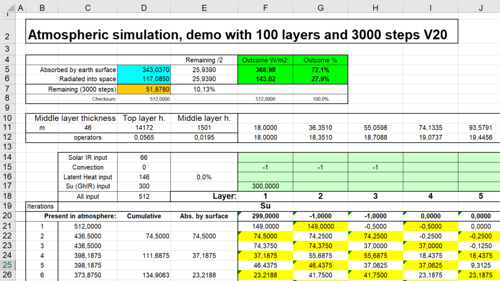
Your main tool to experiment is the input of energy in the atmosphere. Feel free to change the numbers in W/m2 in the soft green area (rows 14 – 17) to match your own estimates.
Row 12 shows the layer thickness, row 11 shows the height of the top of that layer.
The input for surface upward radiation is now 300 W/m2 inserted in layer 1 on position F17.
In this example convection is taking away some energy in the lower layers (F15-H15). Of course the total of this row has to be zero, since all convective energy is released at another place.
All changes you make will immediately result in a new outcome F5, which is the actual greenhouse effect, warming the surface.
Some minor changes were made to the text of this chapter.