One of the assumptions about the way latent heat is radiated into space, is “deep convection”. Like the standard greenhouse theory that was described in chapter 9, this suggests that the main radiation into space is from high in the atmosphere, near or even above the tropopause.
I have always had my doubts about that. As discussed in chapter 9 there is hardly any water vapour and a very low concentration of CO2 at that height, and temperatures are extremely low. With radiation decreasing with the 4th power of the temperature, how can so much energy be disposed of, with so few GHG molecules, at so low temperatures?
I expected that lower parts of the atmosphere would be more important, even for the emission of the energy from deep convection to space. But it was not easy to quantify that without modelling the Hadley Cycle, which is powering most of the latent heat transport (LHT). Still I decided to give it a try, as a showcase of what my Fireworks simulation could do, if provided with the right data by experts.
The Hadley Cells: the worlds cooling engine
As Willis Eschenbach explained so clearly in his presentation at the ICCC4 in 2010, the earth might have a powerful thermostat, consisting of the tenthousands of daily tropical thunderstorms.

They are part of the Hadley cells and transport enormous amounts of latent heat to the tropopause. In the theory of Eschenbach they compensate the radiative effects of greenhouse gas concentration changes, and probably have done so for billions of years.
But how does this Hadley cell actually work? What really drives it, and how does that relate to the standard explanation of the greenhouse effect?
Adiabatic lapse rates
Ascending dry air will expand adiabatically because of the decreasing pressure, which will cool it down with app. 10 degrees per km (see the dry adiabatic lapse rate – DALR – in the third graph of this chapter).
When descending it will follow the same line, warming up.
In the tropics however there is a huge difference between ascending and descending parcels of air.
Because the air at the surface (ocean or rainforest) is close to being saturated with water vapour, it will get saturated immediately as soon as it rises and cools down. This is caused by the maximum amount of water vapour that a parcel of air can hold, which decreases quickly with cooling. Especially at temperatures above 20C.
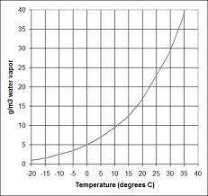
Saturation vs temperature curve
The graph shows that a parcel of air which cools down from 35 C to 20 C looses 50% of it’s water vapour, which condensates into precipitation. While condensating, it releases its latent heat, which of course is equal to the energy that was absorbed while evaporating at the surface.
This released energy heats up the air, making it lighter than it’s environment and increases the upward movement.
The result of the release of the latent heat is that saturated air will only cool down with app. 6C per km in the lower tropopause, instead of 10C as in dry air. Above 10km when almost all water has condensated, it will act as dry air and follow the DALR curve.
So when rising to the same altitude als a dry parcel of air, it will be much warmer.
The released heat also causes it to continue to rise, untill it reaches the warmer air above the tropopause. In fact it will establish a higher tropopause, since the tropopause is determined by the end of the rising of the convection. So rising moist air will push up the tropopause.
Convection cells analysed
Tropical convection always appears above sea or rainforest, with moist air at the surface, so the rising air will follow the saturated adiabatic lapse rate (SALR) until the tropopause. Tropical storms will even break through the tropopause locally and transport energy to up to 18 km high.
Finally the air gets trapped between the cooler troposphere beneath it and the warmer stratosphere above it. Before it can descend, it has to cool down until it can follow the dry adiabatic lapse rate curve.
In the mean time it is not hanging still, but drifting away to the subtropical regions. During this journey the air slowly looses energy by radiating into space:

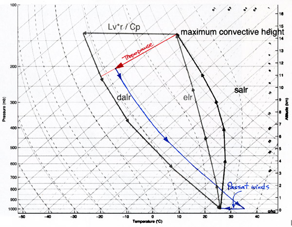
Hadley Cell caught in a diagram
In the diagram you can see how the upward flow ends at 14,5 km high and a temperature of –65 C, following the SALR.
Then it has to stay in the tropopause to loose energy and cool down.
Moving away from the equator, there is less convection, so the tropopause drops (in this case to 11,5 km, and a temperature of –80C). While moving from 14 to 11 km height, it is assumed by some that the latent heat is radiated into space.
Calculating the emissions of the Hadley Cell
Actually, now we have enough information to (roughly) calculate where the cell radiates it’s energy to space, and how much. Because, during the whole cycle, we know:
– from the diagram: the temperature and the height
– from the Fireworks simulation: the part of the energy that is radiated to space at any layer
– from the Fireworks simulation: the height of the layers.
So let’s assume a certain amount of energy being radiated in all directions, by a parcel of air , rising from the surface. When cooling down with height, it will radiate less, with the 4th power. This gives us a measure of the amount of radiation at any temperature, at any height.
At the same time we can calculate with the Fireworks simulation how much of the radiation at any height is radiated to space. In order to do that, I calculated what this radiation ratio was for the SALR and the DALR, for every 500m between the surface and the tropopause, in 30 steps.
I assumed 100 layers in the saturated tropics, and 30 layers in the dry deserts of the subtropics where the main GHG, water vapour, is missing, and tried to find layers that matched the 500 m steps. That gave quite a few mismatches, so there is a lot of “noise” if you would look closely at the data. But the general picture is very smooth:

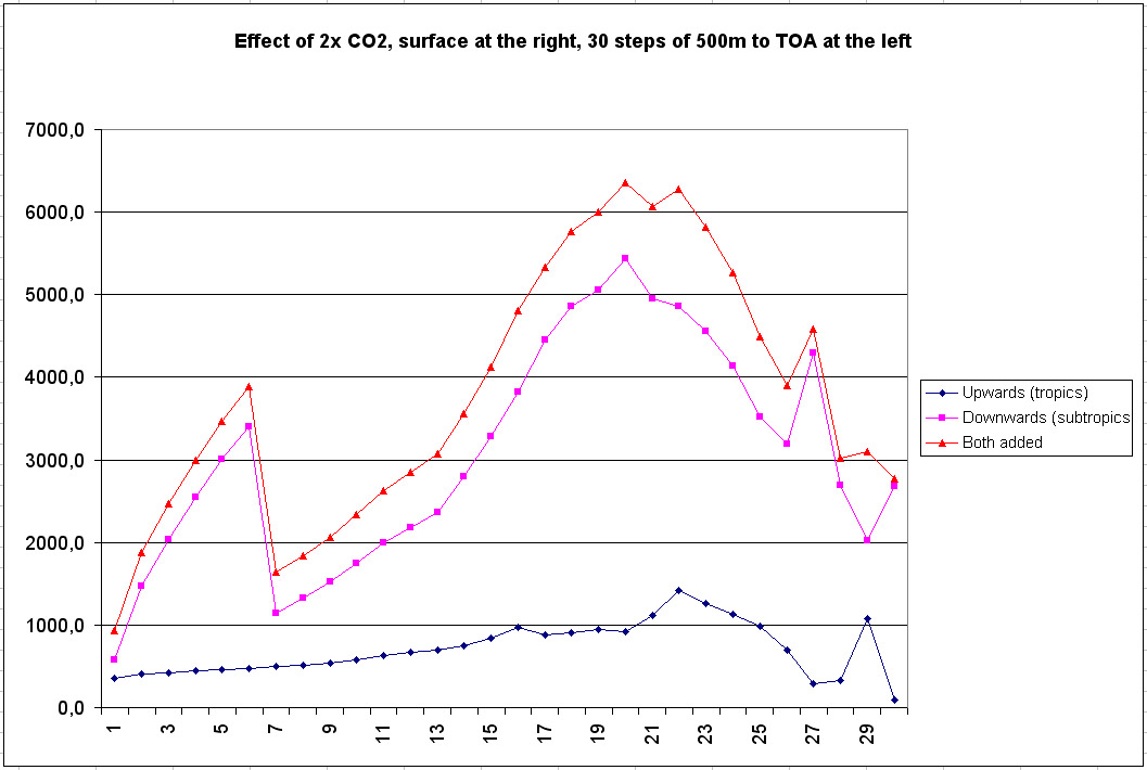
Hadley emission to space
This picture shows the radiation per time unit to space of the greenhouse gases at a specific height.
It has the surface at the right and the tropopause at the left, with 30 steps of 500m. So 5 km height is at step 20 and 1 km height is at step 28.
The rising air (dark blue line) first emits almost everything to the surface (steps 30 to 28), but at 1 km (step 28) it begins to radiate to space, reaching a peak at 4 km (step 22).
Of course a larger part of the radiation will be emitted to space at greater height, but the dropping temperature decreases the radiation itself more, so from 4 km on you see a decrease in emissions to space.
When CO2 doubles, a 114 layer atmosphere is assumed here, resulting in the purple line giving radiation to space.
From this moment on, we assume that the air has lost almost all its water vapour, and will behave as in an atmosphere of 30 layers.
Once trapped at the tropopause, the air has to cool down and descend slowly, following the green line, in steps 1 to 7. This is during the journey to the subtropics.
Then, at 11.5 km (step 7), it is cold enough to descend with the DALR and heat up fast, increasing radiation to space, even though at lower altitude a smaller part of the radiation will reach space. Because there are less layers, the peak is at 2 km high (step 26) this time.
When doubling CO2, the influence is much larger now, since the 30 layers are mainly based on CO2. So for the CO2 influence I chose an increase to 40 layers here (the red line).
Time
This picture needs another factor though. The radiation per time has to be multiplied with the real time that the radiation took place, in order to get the amount of energy that is radiated out. So I chose “1” for the very fast rising of air in the tropical storms, a factor 4 for the much slower descent in the subtropics, and a factor 12 for the period that the air is moving through the tropopause. These factors are not completely random, but I welcome all suggestions for improvement.
If we make a picture with the values multiplied with time, this result appears:
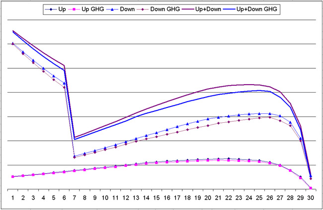
Hadley emission to space x time
This gives a clear view on where the Hadley cell looses it’s energy to space. And as I expected, only a small part (app. 30%) is radiated from the tropopause! Most is radiated to space from 1 to 10 km, peaking between 1,5 and 5 km.
Simplification of surface temperature situation
The calculations are based on the very simple lapse rate diagram in the second illustration of this chapter.
In the diagram the temperature at the surface is assumed to be the same in the subtropics as in the tropics. In reality there will be huge differences.
In the oceans there will not be a significant difference, but deserts are much warmer during the day than rainforests or the ocean.
Considering the desert situation during the day would result in this diagram:
Hadley Cell assuming desert day temps and trade winds
In this diagram you can see that the air will be able to descend earlier and spend less time at the tropopause, and that the temperature of the descending air will be app 10 degrees warmer over the whole downward path, if you assume the surface to be 10 degrees warmer. With desert temperatures of over 50C, the descending air would even be 25 degrees warmer. Considering radiation will increase with the 4th power, this would shift the part of the energy radiated to space even a lot further into the descending path of the Hadley Cell.
This means that the simplification of the surface situation in the calculations keeps me at the safe side of my claims.
Clouds in the fireworks model
The obvious error in this calculation is the complete omission of clouds.
In the general energy balance in chapter 5, clouds are primitively accounted for by a general percentage of sky coverage, but in this Hadley cell analysis, this would not work.
Let’s first look at clouds from the Fireworks Theory point of view.
Translated into its layer definition, clouds represent a part of the atmosphere with an infinite number of layers. So, in an equilibrium situation, only an infinitely small part of the surface upward radiation will be emitted to space after absorption, and all energy will be emitted back to the surface.
Since water or ice particles are not greenhouse gases but behave like black bodies (BB), they absorb the complete IR spectrum (visible light is reflected though), and also the emitted radiation will have a normal BB spectrum. Part of it will pass through the IR window and reach the earth surface without being absorbed.
This results in the effect that we all know: at night, under a cloudy sky, the surface stays much warmer than under a clear sky.
Clouds in the Hadley Cell analysis
Let’s see what the influence of clouds could be on our analysis.
In the downwards part of the cell, there are no clouds, so this part is accurate.
In horizontal movement part of the cell in the tropopause, there are hardly any clouds, and as far as there are, they are very thin cirrus clouds. I don’t know if they are increasing the emission into space or decreasing it: whatever energy they contain or whatever IR they absorb, they will emit as a black body, so the IR window part of the energy will be radiated straight to the earth surface and into space. At the same time they will not absorb visible light, because they reflect it. This will cool down the clouds a lot, thus reducing their emission capacity.
Without suggesting to have any expert knowledge about this complex subject, I don’t expect a considerable influence of clouds on the emission to space in this part of the cell.

Tropical storm
Finally: the rising part of the cell.
This part is heavily influenced by clouds. In fact, the continuous latent heat release over the saturated adiabatic lapse rate is by definition producing clouds.
Since a vertical column of clouds as in a tropical storm is impenetrable for radiation, the only direct emission into space will be from the top of the anvil. But this too has a very low temperature and a low emission.
What about the emission during the upward movement, in our graph represented by the low bent curve, representing app. 30% of the total emission into space according to that graph?
It is obvious that at the location of a tropical storm, there will not be any radiation into space, apart from the anvil, ic the last layer.
There are a number of reasons why there still is emission into space at lower levels:
– The tropical storms only cover a part of the surface
– The tropical storms only form during the day, finally producing the anvil. Until that moment, there is radiation from lower levels, and that is substantial because of the higher temperature and the BB spectrum of clouds.
– The vertical column of clouds of a tropical storm emits its energy to the air around it. This air will behave like a normal moist atmosphere and emit its energy into space.
Considering all this, it is, in my opinion, likely that omitting clouds in the analysis, results in a too high estimation of the emission during the upwards part of the cell. If this error is 20 or 80% is hard to tell. My guess is between 40 and 60%.
This would not significally affect my conclusion.
Greenhouse effect
Now let’s see what CO2 is doing, by subtracting the two curves:
Decrease of latent heat, radiated into space in the Hadley cell, caused by CO2 doubling
Here the noise in the data shows more clearly, but the conclusion is obvious: the influence of CO2 doubling on the radiation to space from the Hadley cell is mainly found between 3 and 7 km high, peaking at 5km, during the descending part of it, in the subtropics.
This supports my claim in chapter 9 that the standard greenhouse theory is erroneous, since it is based on the assumption that the energy is radiated to space from the tropopause, right above the place from where it was transported upwards.
Actual measurement data check
These findings should not come as a surprise: when you look at the latent heat and outgoing long wave radiation (OLR) maps, it is obvious that where the Latent heat is transported upwards, it is not radiated into space.
First the latent heat transport (LHT), which is mainly found above the oceans and the rainforests, but not at all at the rest of the continents:

Latent heat flux
In the deserts however, where there is absolutely no LHT, but the downward part of the Hadley cells, there you find the maximum OLR:

OLR
The standard greenhouse theory would suggest that both have to occur at the same place, since the ALR, which is supposed to be pushed up by the tropopause, is a local phenomenon.
It seems to me that my calculations, although still based on weak data, are much more convincing, since they are supported by observations.
Is CO2 increase heating up the atmosphere after all?
In this chapter we established an influence of CO2 increase on the radiation during the Hadley cycle, which leads to a decrease of emission to space over the whole loop. This seems to contradict the thermostat theory of Willis Eschenbach, and chapter 7, where I suggested that doubling CO2 has (also) a direct cooling influence by increasing convection.
But it should be noted that, for the purpose of analysis, I calculated the radiative aspect of a Hadley Cell that was assumed to be completely unaffected by the CO2 content or the temperature changes that might occur. With convection and latent heat transport kept constant, the results could be compared.
However, the cell itself is of course influenced by the heating and cooling aspects of the GHG.
As was calculated in chapter 5, an increase of 1 degree in surface temperature (by any cause), would be compensated by less than 1% increase in latent heat transport. So the calculated influence of CO2 would be fully compensated as soon as it comes with a tiny change in convection.
Conclusions
This Hadley cell analysis shows us that most of the latent heat that is transported upwards in the tropics, is radiated into space in the subtropics, from an altitude of 1,5 to 5 km. Only for a minor part it is radiated into space from the tropopause, while floating to the subtropics.
This means that the standard greenhouse gas effect explanation is wrong.
The analysis does not prove the existance of a thermostat in the Hadley cell.
On the other hand, it is consistent with the presence of the tropical thunderstorm thermostat as described in the hypothesis of Eschenbach.
Added on June 8th
Two paragraphs:
– Clouds in the fireworks model
– Clouds in the Hadley Cell analysis
Added the red line (=addition of upward and downward effect) in the graph “Hadley GHG influence x time”
Chapter 10 was partially revised, and some graphs were replaced or added.
Some minor changes have been made to this chapter.
Hi Sir,
Is that true that mean streamline functions are really useful to know the Hadley cell (HC) dynamics as the averages of averages will relinquish several trends of HC?
I want to know how to calculate the Hadley Circulation index?
Dear Mr Sree,
I don’t know to what degree my calculation could help to describe other functions in the HC than radiation. It is of course an extremely simplified model.
But in my opinion it was accurate enough to serve my purpose: calculating where the largest part of the latent energy of the cycle is emitted out of the atmosphere. Even despite the huge inaccuracies that are still in it, I think I made quite plausible that most energy is radiated out in the descending part of the HC.
This proves the general greenhouse gas theory wrong, as is described in chapter 9.
Regards,
Theo Wolters